Morphological Analyses
This section should give you an impression of how to access and compute morphological properties of neurons. You will note that most of this uses navis functions. CatmaidNeuron/Lists are fully compatible with navis and you should most definitely check out tutorials on its docs.
Basic properties
Many basic parameters are readily accessible through attributes of CatmaidNeuron or CatmaidNeuronList:
[1]:
import pymaid
import matplotlib.pyplot as plt

rm = pymaid.CatmaidInstance('server_url', 'api_token', 'http_user', 'http_password')

nl = pymaid.get_neurons('annotation:glomerulus DA1 right excitatory')

# Access single attribute: e.g. cable lengths [um]
nl.cable_length
INFO  : Global CATMAID instance set. (pymaid.fetch)
INFO  : Looking for Annotation(s): glomerulus DA1 right excitatory (pymaid.fetch)
INFO  : Found 8 skeletons with matching annotation(s) (pymaid.fetch)
[1]:
array([1591.51982146, 1182.10245803, 1035.09925403, 1113.15667872,
       1215.92059396, 1182.6479815 , 1059.72905251, 1109.88615456])
[2]:
# .. or get a full summary as pandas DataFrame
df = nl.summary()
df.head()
[2]:
| neuron_name | skeleton_id | n_nodes | n_connectors | n_branch_nodes | n_end_nodes | open_ends | cable_length | review_status | soma | |
|---|---|---|---|---|---|---|---|---|---|---|
| 0 | PN glomerulus DA1 27296 BH | 27295 | 9969 | 463 | 211 | 218 | 58 | 1590.676589 | NA | True |
| 1 | PN glomerulus DA1 57312 LK | 57311 | 4874 | 421 | 156 | 163 | 105 | 1180.597489 | NA | True |
| 2 | PN glomerulus DA1 57324 LK JSL | 57323 | 4585 | 434 | 120 | 127 | 59 | 1035.076857 | NA | True |
| 3 | PN glomerulus DA1 57354 GA | 57353 | 4895 | 324 | 90 | 95 | 52 | 1113.156676 | NA | True |
| 4 | PN glomerulus DA1 57382 ML | 57381 | 7727 | 357 | 153 | 162 | 71 | 1215.920594 | NA | True |
Rerooting, resampling, simplifying
navis lets you perform (virtual) surgery on neurons. Many of the base functions are also accessible directly via CatmaidNeuron and CatmaidNeuronList methods. E.g. pymaid.CatmaidNeuronList.resample() is simply calling navis:navis.resample_neuron().
Examples continue from above code.
[3]:
# Reroot a single neuron to its soma
nl[0].soma
[3]:
3005291
[4]:
# .soma returns the treenode ID of the soma (if existing) and can be used to reroot
nl[0].reroot(nl[0].soma, inplace=True)
[5]:
# You can also perform this operation on the entire CatmaidNeuronList
nl.reroot(nl.soma, inplace=True)
Above code is equivalent to:
[6]:
import navis
navis.reroot_skeleton(nl, nl.soma, inplace=True)
We will be using the shortcut (e.g. nl.reroot) and the actual function (e.g. navis.reroot_skeleton) interchangeably throughout the examples. This is not meant to be confusing but to be illustrative.
If you work with large lists you may want to down-/resample before e.g. plotting.
[7]:
# Downsample by "skipping" N nodes (here: 10)
nl_downsampled = navis.downsample(nl, 10, inplace=False)
# More elaborate: resample to given resolution in nanometers (here: 1000nm = 1um)
nl_resampled = navis.resample_skeleton(nl, 1000, inplace=False)
[8]:
import matplotlib.pyplot as plt

# Plot an original neuron first
fig, ax = navis.plot2d(nl[0], color='red')

# Shift the downsampled and resampled versions slightly and plot
n_ds = nl_downsampled[0].copy()
n_rs = nl_resampled[0].copy()

n_ds.nodes.x += 10000
n_rs.nodes.x += 20000

fig, ax = n_ds.plot2d(color='blue', ax=ax)
fig, ax = n_rs.plot2d(color='green', ax=ax)

plt.show()
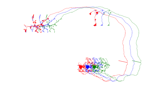
Looking closely, you will find that the downsampled (blue) and resampled (green) neurons are smoother.
Important
Note how we used inplace parameter when using the neuronlist’s downsampling method?
This parameter works like in pandas: if True will perform the action on the neuronlist, if
False will operate on and return a copy and leave the original neuronlist unchanged.
Cutting, pruning, pasting
Examples continue from above code.
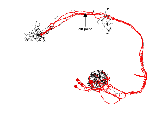
[9]:
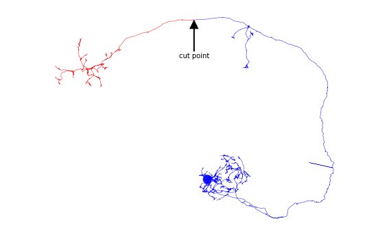
# Cut a neuron in two using either a node ID or (in this case) a node tag
distal, proximal = navis.cut_skeleton(nl[0], cut_node='SCHLEGEL_LH')

# Plot neuron fragments
fig, ax = navis.plot2d(distal, color='red', method='2d', connectors=False)
fig, ax = navis.plot2d(proximal, color='blue', method='2d', connectors=False, ax=ax)

# Annotate cut point
cut_coords = distal.nodes.set_index('node_id').loc[ distal.root, ['x','y'] ].values[0]
ax.annotate('cut point', xy=(cut_coords[0], -cut_coords[1]),
            xytext=(cut_coords[0], -cut_coords[1]-20000), va='center', ha='center',
            arrowprops=dict(facecolor='black', shrink=0.01, width=1),
            )

plt.show()
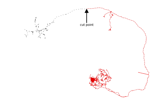
Instead of cutting a neuron in two, we can also just prune bits off a neuron objects:
[10]:
n = nl[0].prune_distal_to('SCHLEGEL_LH', inplace=False)

# Plot original neuron in black
fig, ax = nl[0].plot2d(color='black', method='2d', connectors=False, linestyle=(0, (5, 10)))

# Plot pruned neuron in red
fig, ax = n.plot2d(color='red', method='2d', connectors=False, ax=ax)

# Annotate cut point
ax.annotate('cut point', xy=(cut_coords[0], -cut_coords[1]),
            xytext=(cut_coords[0], -cut_coords[1]-20000), va='center', ha='center',
            arrowprops=dict(facecolor='black', shrink=0.01, width=1),
            )

plt.show()
[11]:
# To undo, simply reload the neuron from server
nl[0].reload()
[12]:
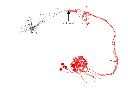
# These operations can also be performed on a collection of neurons
n = nl[:5].prune_distal_to('SCHLEGEL_LH', inplace=False)

# Plot original neurons in black
fig, ax = nl[:5].plot2d(color='black', method='2d', connectors=False, linestyle=(0, (5, 10)))

# Plot pruned neurons in red
fig, ax = n.plot2d(color='red', method='2d', connectors=False, ax=ax)

# Annotate cut point
ax.annotate('cut point', xy=(cut_coords[0], -cut_coords[1]),
            xytext=(cut_coords[0], -cut_coords[1]-20000), va='center', ha='center',
            arrowprops=dict(facecolor='black', shrink=0.01, width=1),
            )

plt.show()
[13]:
# Again, let's undo
nl.reload()
nl.reroot(nl.soma)
[14]:
# Something more sophisticated: pruning by strahler index
n = nl[:5].prune_by_strahler( to_prune = [1,2,3], inplace=False )

# Plot original neurons in black
fig, ax = nl[:5].plot2d(color='black', method='2d', connectors=False)

# Plot pruned neurons in red
fig, ax = n.plot2d(color='red', method='2d', connectors=False, ax=ax, linewidth=1.5)

# Annotate cut point
ax.annotate('cut point', xy=(cut_coords[0], -cut_coords[1]),
            xytext=(cut_coords[0], -cut_coords[1]-20000), va='center', ha='center',
            arrowprops=dict(facecolor='black', shrink=0.01, width=1),
            )

plt.show()
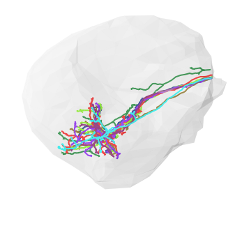
We can also intersect neurons with CATMAID volumes:
[15]:
# Again, let's undo
nl.reload()
[16]:
# Get a volume
lh = pymaid.get_volume('LH_R')

# Prune by volume
nl_lh = navis.in_volume(nl, lh, inplace=False)
[17]:
# Set color of volume
lh['color'] = (250,250,250,.2)

# Plot neurons that have some cable left and the volume
fig, ax = navis.plot2d([nl_lh[nl_lh.cable_length > 10], lh],
                       method='3d',
                       connectors=False,
                       linewidth=2)

ax.dist=6
plt.show()
And now go check out navis!