Plotting

pymaid piggy-backs on navis for 2D and 3D plotting of neurons. This notebook will give you a introduction but you should check out navis docs for more in-depth tutorials.

Neuron objects, CatmaidNeuron and CatmaidNeuronList have built-in methods that call navis.plot3d() or navis.plot2d().

2D Plotting

This uses matplotlib to generate 2D plots. The big advantage is that you can save these plots as vector graphics. Unfortunately, matplotlib’s capabilities regarding 3D data are limited. The main problem is that depth (z) is at best simulated by trying to layer objects according to their z-order rather than doing proper rendering. You have several options to deal with this: see method parameter in navis.plot2d(). It is important to be aware of this issue as e.g. neuron A might be plotted in front of neuron B even though it is actually spatially behind it. The more busy your plot and the more neurons intertwine, the more likely this is to happen.

import pymaid
import matplotlib.pyplot as plt

# Connect to CATMAID
rm = pymaid.connect_catmaid()
# Get two example neurons by their skeleton ID
nl = pymaid.get_neurons(['57311', '27295'])

# Plot using default settings
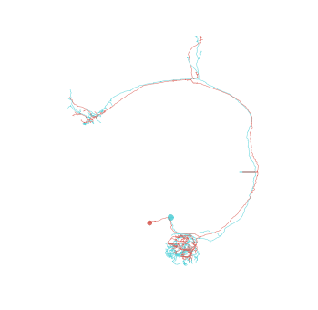
fig, ax = nl.plot2d()
plt.show()

INFO  : Global CATMAID instance set. Caching is ON. (pymaid)

Above plot used the default matplotlib 2D plot. This is very fast and convenient to get an impression of a neuron’s morphology.

Under the hood nl.plot2d is actually calling navis.plot3d() - this works because pymaid.CatmaidNeuron is a subclass of navis.TreeNeuron and any navis function that works with TreeNeurons also works with CatmaidNeurons or lists thereof. Hence, we could also do this:

import navis

# Plot using default settings
fig, ax = navis.plot2d(nl)
plt.show()

Matplotlib has some basic 3D plotting capabilities that are perfectly sufficient for simple visualizations but are limited when it comes to perspectively correct z-ordering. Not perfect but this “2.5D” allows us to rotate neurons:

# Plot using matplotlib's 3D capabilities
fig, ax = navis.plot2d(nl, method='3d_complex')
# Change from default frontal view to lateral view
ax.azim = 0
# Zoom in a bit
ax.dist = 6
plt.show()

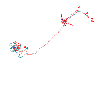
Noticed how we changed the perspective by adjusting the azimuth (.azim)? You can also change the elevation (.elev) to get a top view.

This can even be used to generate small animations:

# Render 3D rotation
fig, ax = navis.plot2d(nl, method='3d_complex')

for i in range(0, 360, 10):
   # Change rotation
   ax.azim = i
   # Save each incremental rotation as frame
   plt.savefig('frame_{0}.png'.format(i), dpi=200)

Plotting volumes

navis.plot2d() and navis.plot3d() are capable of visualizing neurons and volumes but can also plot scatter plots. You can combine multiple objects by passing them as a simple list []:

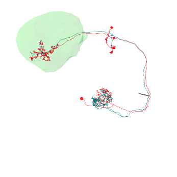
# Retrieve volume
lh = pymaid.get_volume('LH_R')
# Set color and alpha
lh.color = (0, 1, 0, .1)
# Plot
fig, ax = navis.plot2d([nl ,lh], method='3d_complex')
ax.dist = 6
plt.show()

Interactive 3D Plotting

For 3D plots, we are using either Vispy (default) or Plotly to render neurons and volumes.

Important

In general, you want to use Vispy if you are using the terminal or an IDE, and Plotly if you are working with Jupyter notebooks. Please note that Vispy currently simply does NOT work within Jupyter notebooks.

By default, navis will detect whether you are working in a Jupyter notebook or not, and choose the correct backend automatically: Vispy for terminal, Plotly for Jupyter. For demonstration purposes, we will override this by using the backend parameter of navis.plot3d().

Our first two example use Vispy:

# Plot using Vispy (will open 3D viewer)
viewer = nl.plot3d(backend='vispy')
# Save screenshot
viewer.screenshot('screenshot.png', alpha=True)

Note

Vispy itself uses either one of these backends: Qt, GLFW,SDL2, Wx, or Pyglet. By default, navis installs and sets PyQt5 as vispy’s backend. If you need to change that use e.g. vispy.use(app='PyQt4')

The navis.Viewer is persistent and survives simply closing the window. Calling navis.plot3d() again will add objects to the canvas and open it again.

# Add another set of neurons to existing canvas
nl2 = pymaid.get_neurons([987675, 543210])
nl2.plot3d(backend='vispy')

# To clear canvas either pass parameter when plotting...
nl2.plot3d(clear3d=True)

# ... or call function to clear
navis.clear3d()

# To wipe canvas from memory
navis.close3d()

If working with multiple viewers, you can specify which :class:`navis:navis.Viewer` to add the neurons to.

# Open 2 iewers
v1 = navis.Viewer()
v2 = navis.Viewer()

# Add neurons to each one separately
v1.add(nl)
v2.add(nl2)

# Clear one viewer
v1.clear()

# Close the second viewer
v2.close()

If you've lost track of your viewer, simply use :func:`navis:navis.get_viewer` to get it back:

v = navis.get_viewer()

Now let’s have a look at Plotly as backend:

# Using plotly as backend generates "inline" plots by default (i.e. they are rendered right away)
fig = nl.plot3d(backend='plotly', connectors=True, width=1000)

Navigating the 3D viewer

1. Rotating: Hold left mousebutton

2. Zooming: Use the mousewheel or hold left+right mousebutton and drag

3. Panning: Hold shift + left mousebutton

4. Perspective: Hold shift + left and right mousbutton

5. Hide/unhide: Click legend (Vispy only)

Adding volumes

navis.plot3d() allows plotting of volumes (e.g. neuropil meshes). It’s very straight forward to use meshes directly from your CATMAID Server: There is a custom class for CATMAID Volumes, navis.Volume which has some neat methods - check out its reference.

# Provide colors
vols = [pymaid.get_volume('LH_R', color=(255, 0, 0, .2)),
        pymaid.get_volume('LH_L', color=(0, 255, 0, .2))]
fig = navis.plot3d([nl, *vols], backend='plotly', width=1000)

You can also pass your own custom volumes:

cust_vol = navis.Volume(vertices=[[1, 2, 1],
                                   [5, 6, 7],
                                   [8, 6, 4]],
                        faces=[(0, 1, 2)],
                        name='custom volume',
                        color=(255, 0, 0))
fig = navis.plot3d(cust_vol, backend='plotly', width=1000)